
Taipei PM2.5 Example
1. Set CRS(Coordinate Reference System)
Select WGS84(EPSG:4326) in “Coordinate Reference System Selector”
2. Specify data
Specify Hard data and Soft data in “Specify Data” window
i. Hard data
Select “PM2.5_105_taipei.csv” from downloaded example file under “/data”
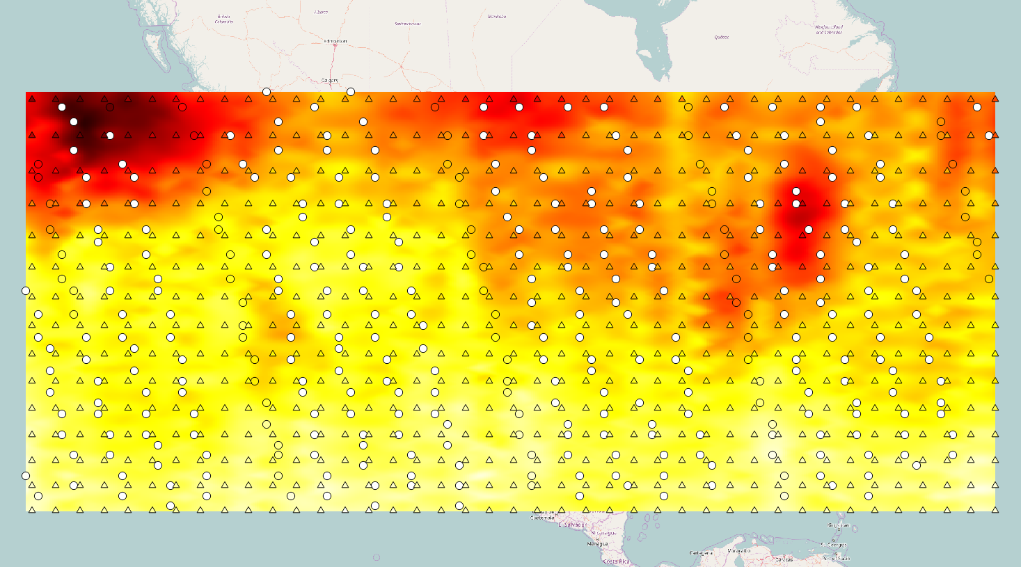
After import hard data and soft data. BMEobj will be created,soft data and hard data will be load in QGIS.

Figure2.1
Time View of hard data

Hard data (circle) and is showed. From figure2.1, color bar and time bar of data are showed on the left and below of figure.
3. Compute Trend and Residual From Data
User can choose “No Detrending”, “Kernel Smoothing” or “STmean” in this step. In this example, we will use “STMean”.
4. Covariance Analysis
4.1 Empirical Covariance Estimation
For this case, we will set:
Spatial Distance Limit: 0.1179 Temporal Distance Limit: 11700.0
Number of Spatial Lags:8 Number of Temporal Lags:8
Spatial Lag Tolerance:0.01684 Spatial Temporal Tolerance: 1671.0
And press “Plot Empirical Covariance”.

And press “Plot Empirical Covariance”.

4.2 Covariance Model Fitting
In this case, we will use “Exponential” to fit covariance. After fitting covariance, 2D and 3D Fit covariance will be plotted.
Nest Number = 2
Fit Covariance Model
C1 =1.164, S1 = 0.05624, T1 =3326
C2 = 0.1365, S2 = 0.03682, T2 = 1861
5. Prediction
Specify location: For this case, we use “Grid Input”, which STARBME will generate grid coordinate for predict. Press “Predict” for predict the coordinate that generate by “Grid Input”, we will set coordinate boundary by select “ Set By Data Boundary”
For Grid Input,
Xn = 80
Yn = 80
Tmin = 0, Tmax = 100, Tn = 101
For Predict,
Order = ZeroMean
Spatial Range = 0.05624
Temporal Range = 3326.0
Spatial/Temporal Ratio = 1.691e-05
Nhmax = 5, nsmax = 0
6. Output result
Specify Task for result: Add Result to QGIS.